Getting SED data¶

The Data access section of mmdc.am builds the multiwavelength spectral energy distribution (SED) of any sky position from radio to gamma rays, with the epoch of every point, and lets you explore it, filter it in time and download it.

Open Data access on mmdc.am

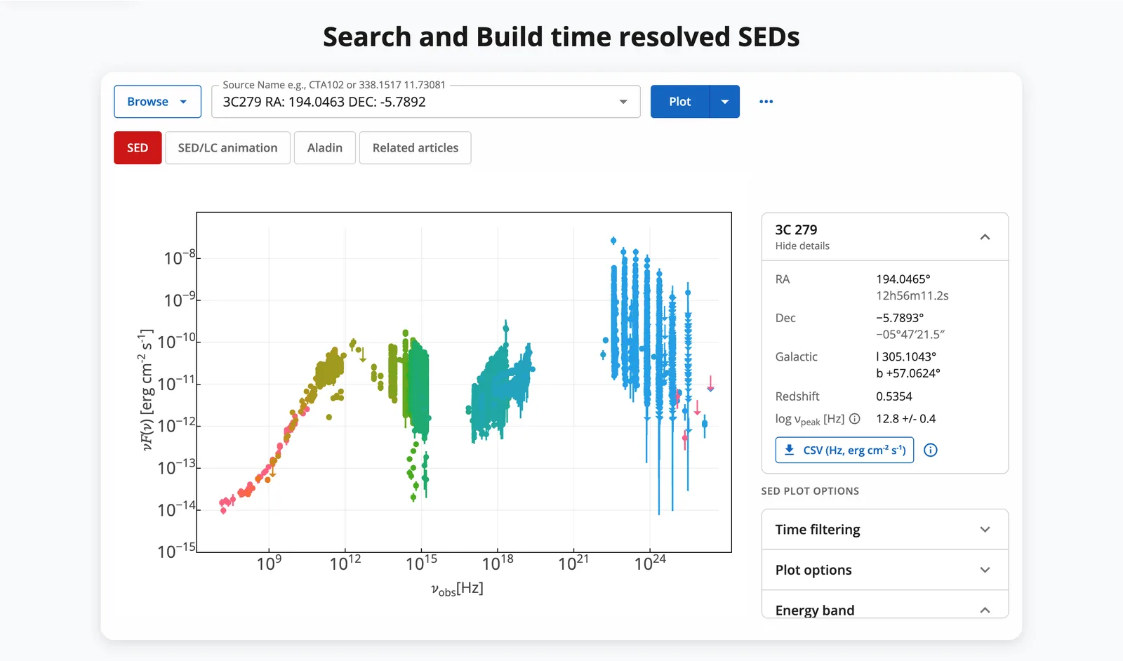
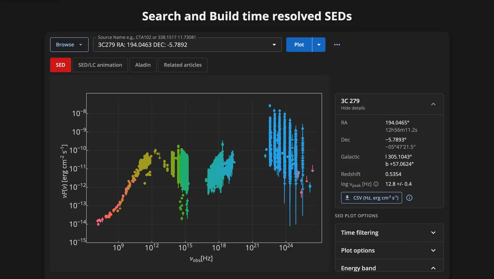
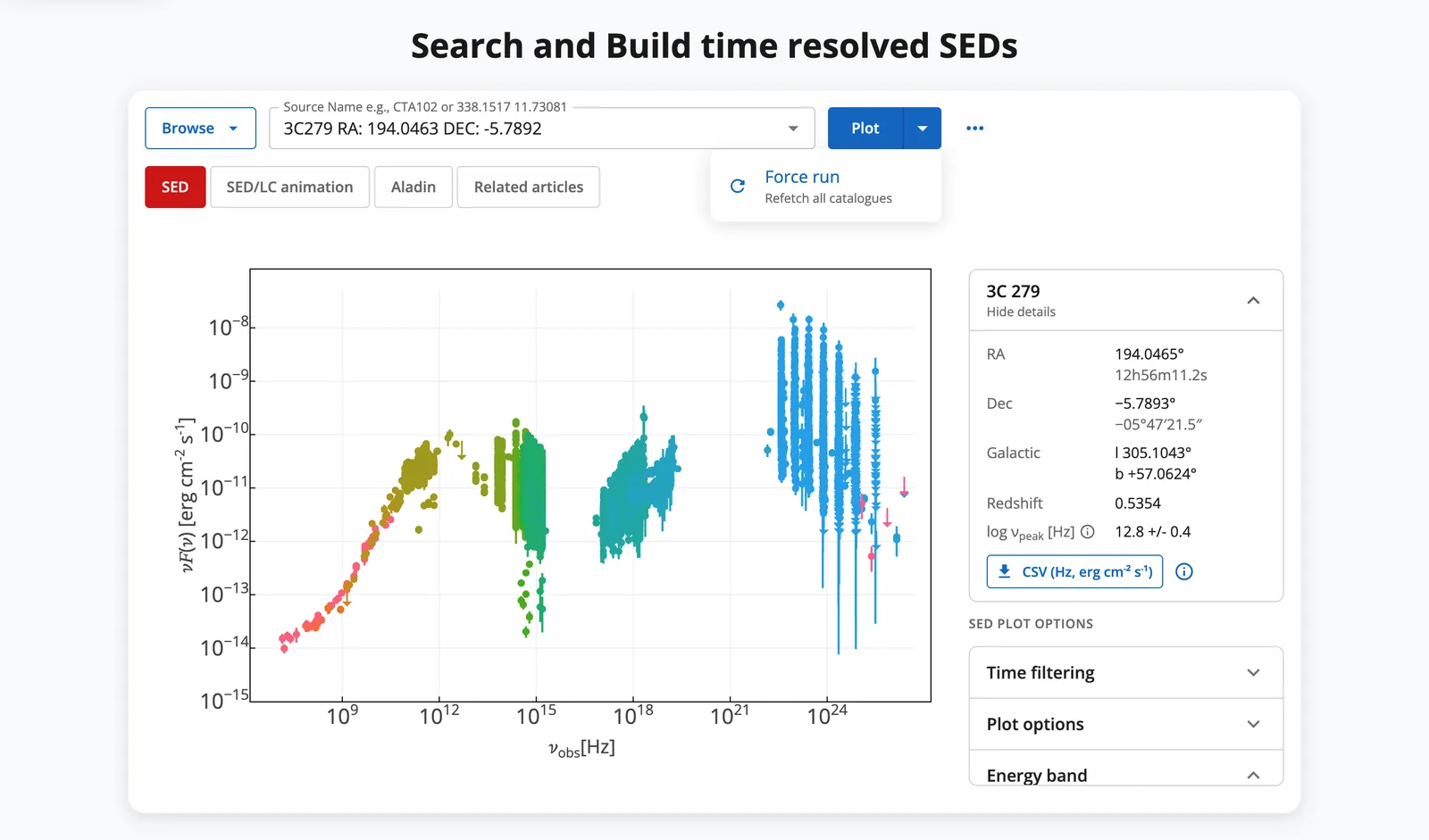
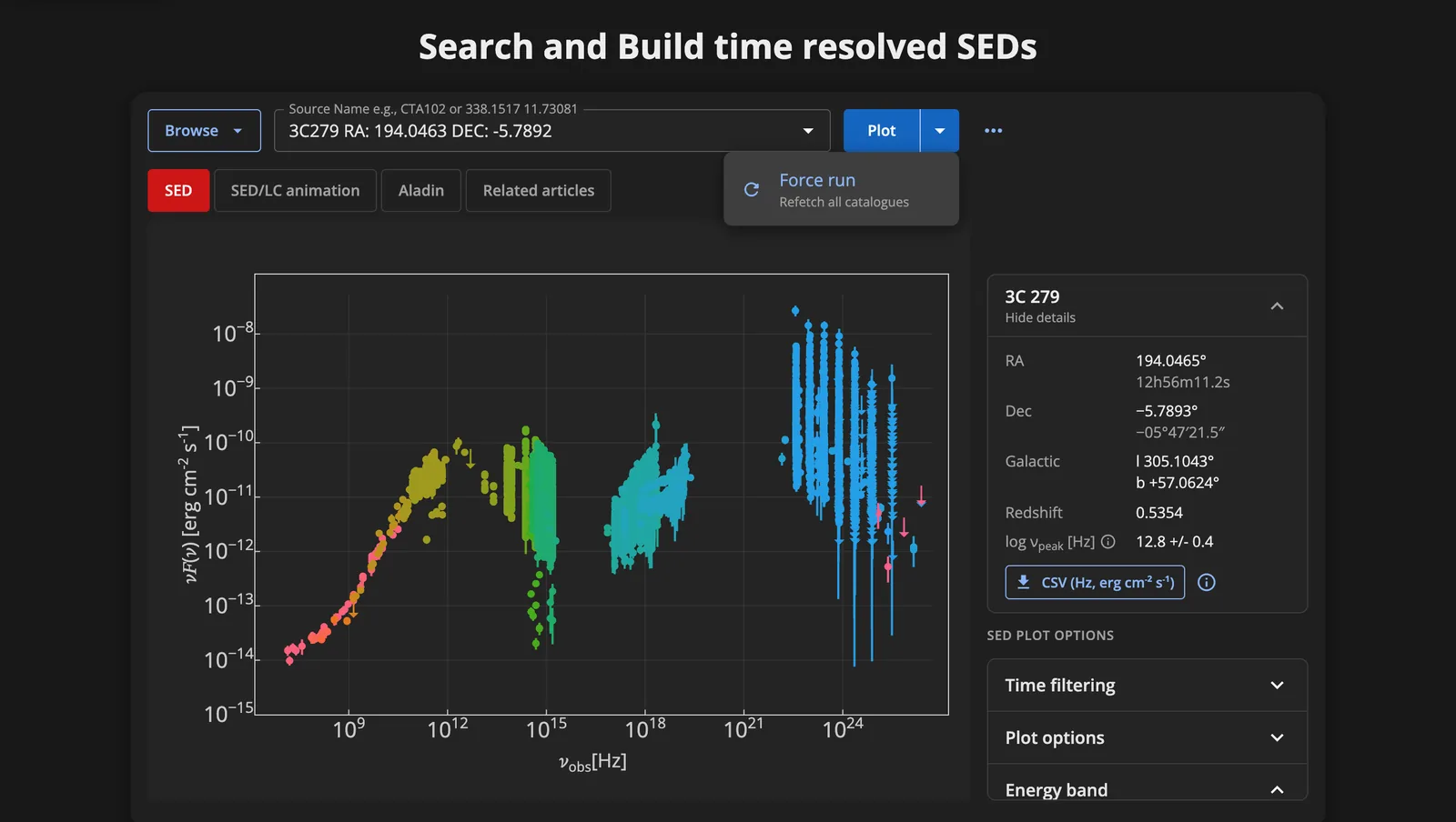
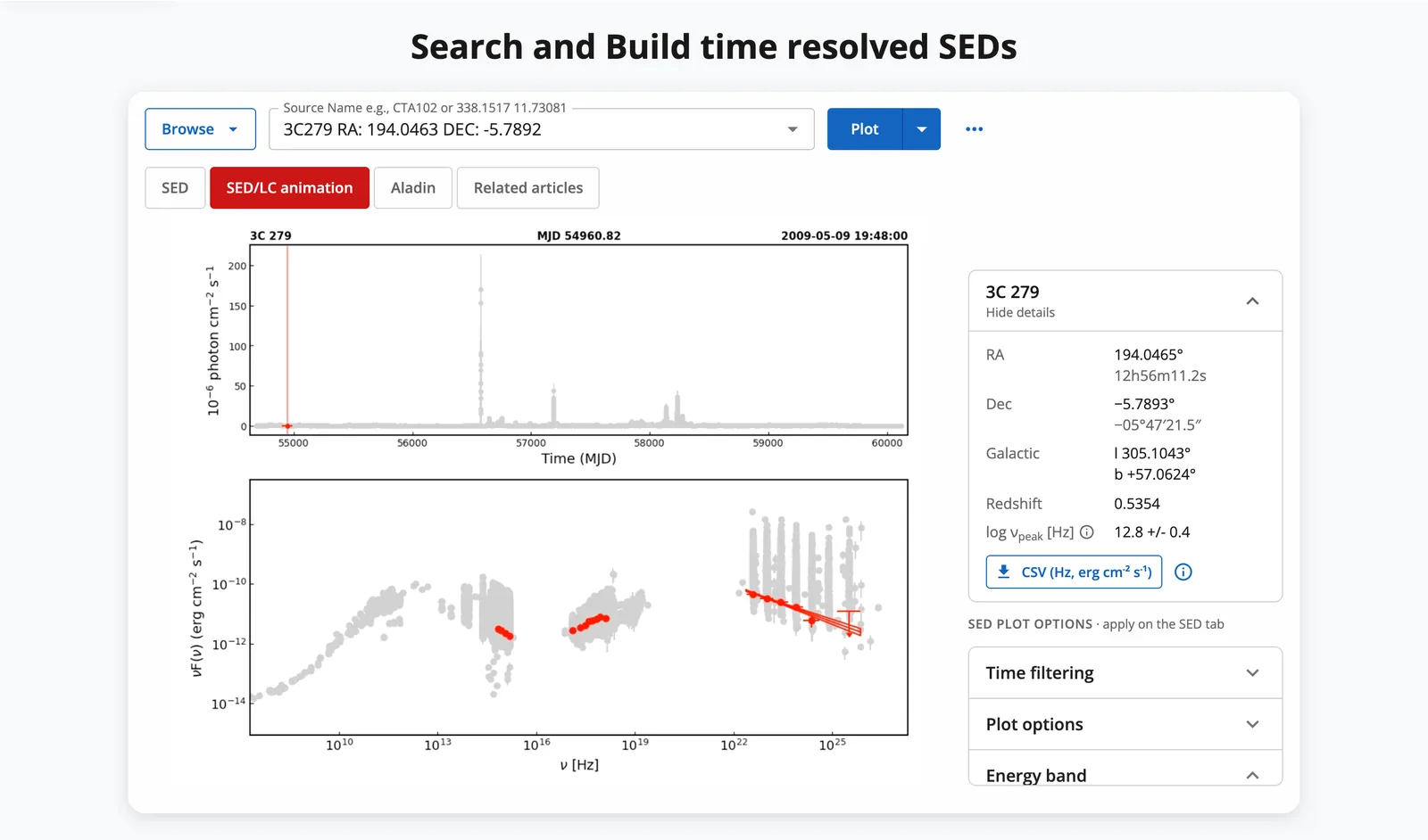
The SED of 3C 279. Left: the SED and its tabs. Right: the source card and the SED plot options.

In short¶

Type a source name and pick it from the list, or type RA Dec in degrees.
Press Plot.
Explore the plot; narrow it with Time filtering and Energy band.
Download the points with the CSV button in the source card.

1. Choose a source¶

The source field accepts:

You type	Example	What happens
A name	`Mrk 421`, `CTA102`	After three characters a list of matching sources appears; pick one. Case and spaces do not matter.
RA Dec in degrees	`338.1517 11.73081` or `338.1517, 11.73081`	Plot is enabled at once, no pick needed. RA from 0 to 360 (360 excluded), Dec from −90 to 90.

A typed name alone is not enough: pick it from the list (or press Enter to take the first match), otherwise Plot stays disabled.

Names are matched in a catalogue originally developed for the Open Universe platform. A name not found there is resolved with NED, then SIMBAD. Catalogue coordinates can differ slightly from NED's; if a search returns nothing, try the NED coordinates instead.

Browse the blazar lists¶

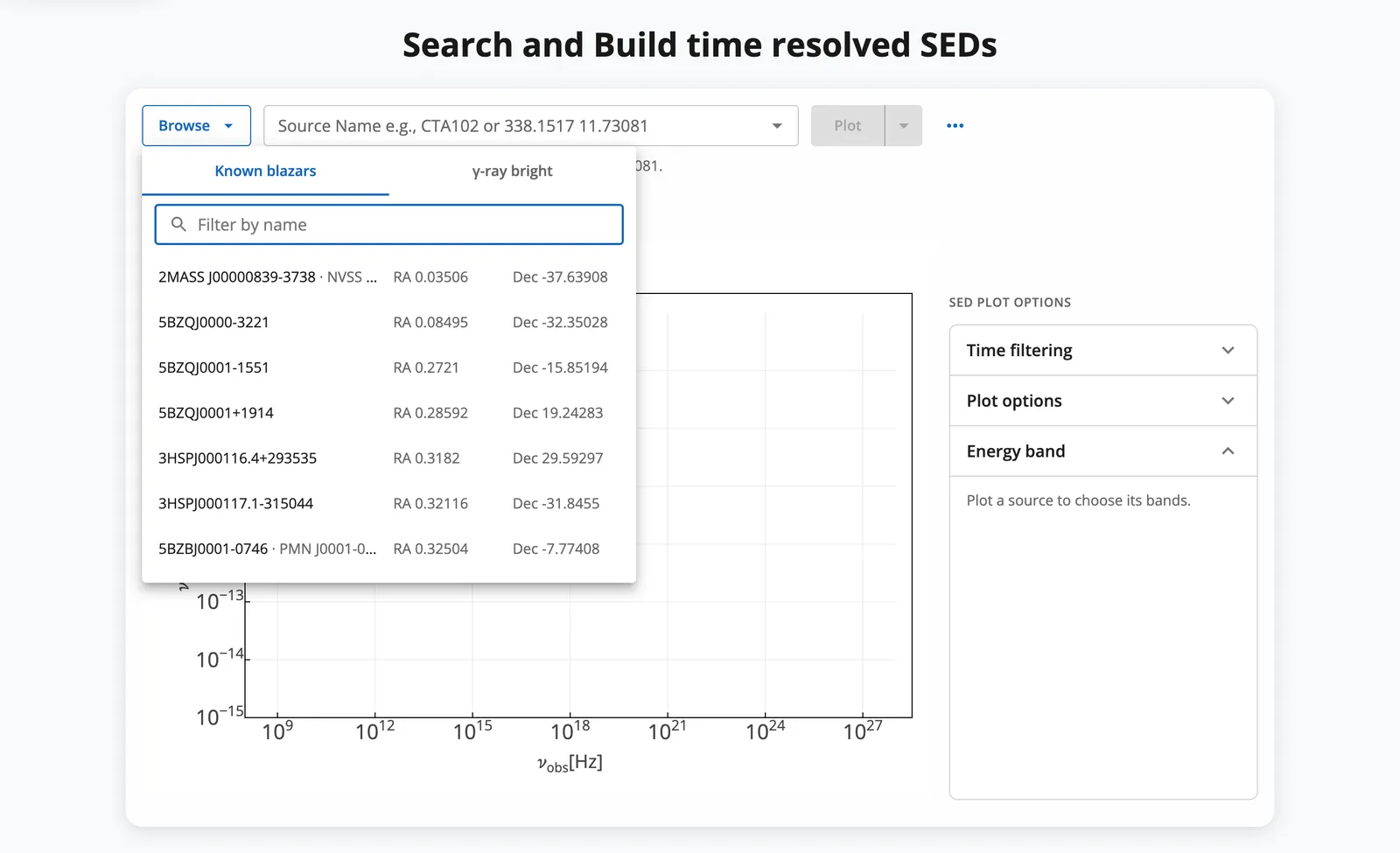
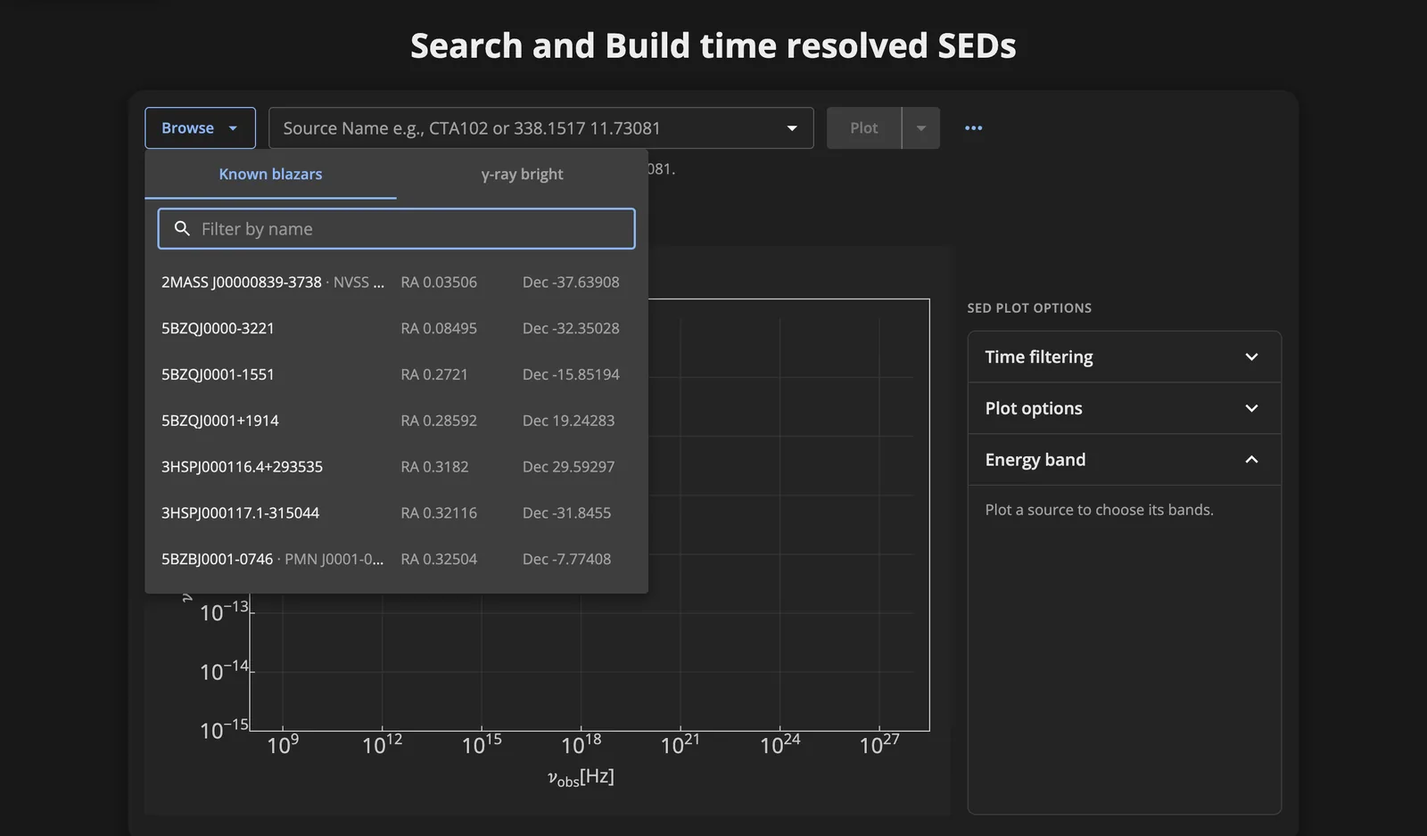
Browse opens two ready-made lists:

Known blazars: about 6,700 blazars from the 5BZCAT, 3HSP and Fermi-LAT catalogues.
γ-ray bright: about 3,400 γ-ray bright blazars, for which MMDC also has SEDs computed over many periods.

Filter a list by name, then click a row: it fills the source field. Press Plot to build the SED.

2. Plot¶

Press Plot. Two cases:

The position was searched before (by anyone, within 2″): the stored SED is shown at once.
A new position: MMDC searches about 75 catalogues and archives (most from copies kept at MMDC, the rest queried live). A progress bar shows each stage (searching X-ray and radio catalogues, the other catalogues, light curves, combining the data). This can take a few minutes.

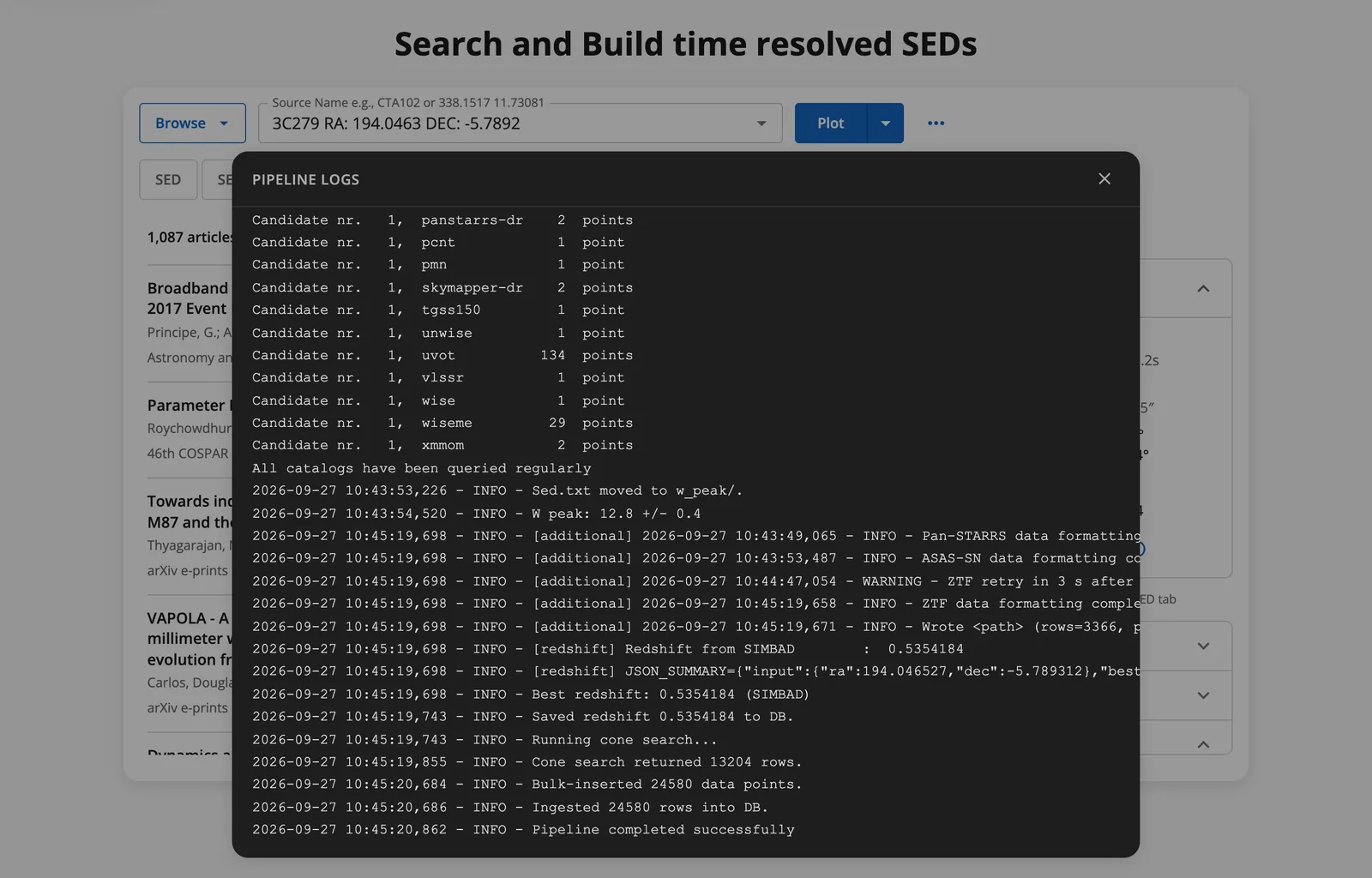
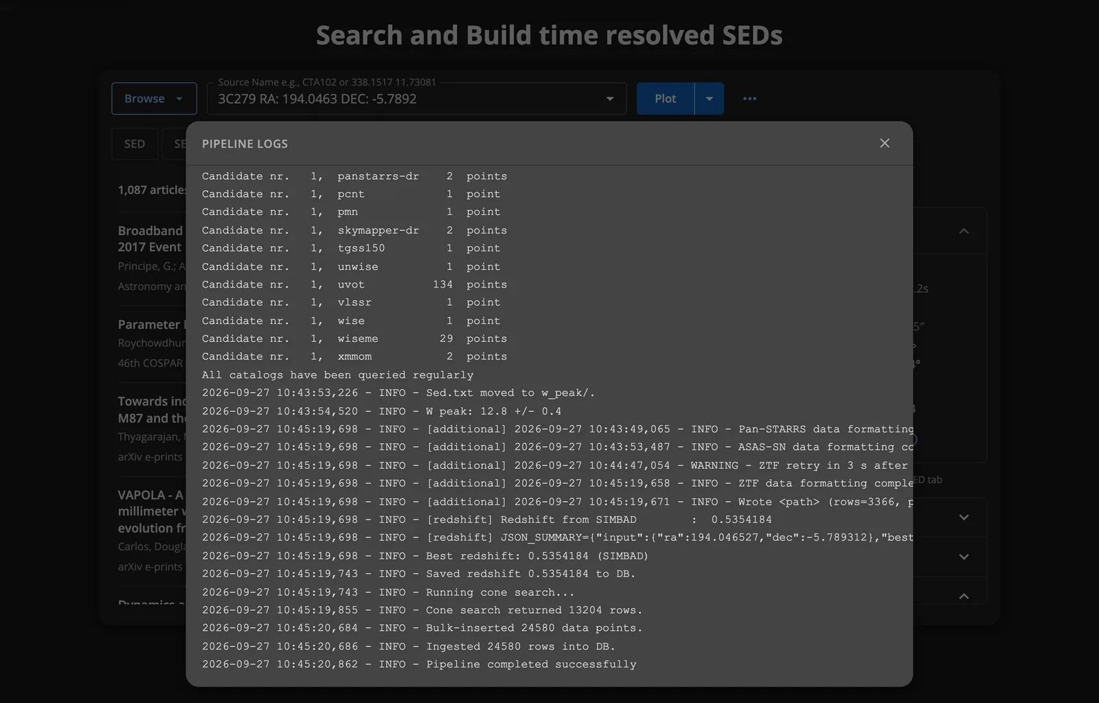
To follow a run in detail, open ⋯ → Show logs. The log lists every catalogue queried and the number of points it returned.

Force run¶

Plot ▾ → Force run fetches every catalogue again instead of using the stored SED. Use it when the last run's logs show that some catalogues were unreachable. When catalogues could not be queried, a notice above the plot names them and offers View logs and Re-run (force). While a re-run is going on, the previous SED stays on screen.

3. Explore the SED¶

The plot is interactive: hover a point for its values, drag to zoom, double-click to reset. Upper limits are drawn as arrows. The camera icon in the plot's toolbar saves a PNG.

The source card¶

The card beside the plot shows:

Field	Meaning
RA, Dec	J2000, in degrees and sexagesimal
Galactic	Galactic longitude l and latitude b
Redshift	From NED, SIMBAD or other catalogues, when one is known
log ν_peak [Hz]	Peak frequency of the synchrotron emission, estimated from the source's WISE/NEOWISE infrared data when they are not dominated by emission unrelated to the jet. "> 17.5" is a lower limit; "—" means no estimate.

SED plot options¶

The panel under the card has three sections; one is open at a time.

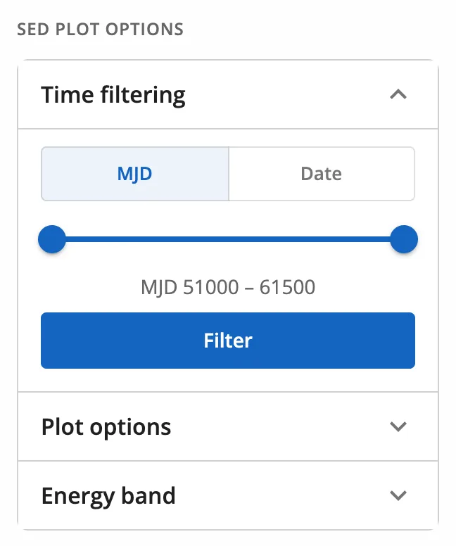
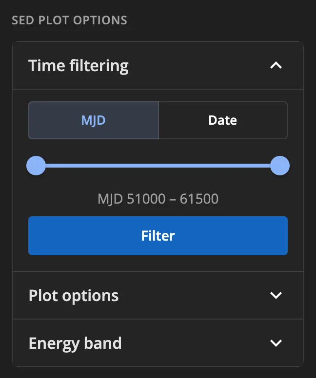
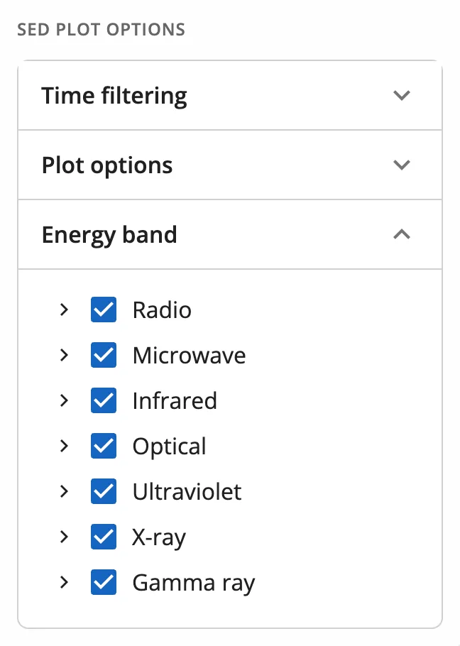
Time filtering keeps only the points observed in a time window. Choose MJD (a slider from MJD 51000 to 61500) or Date (two calendar dates), then press Filter. Points without an observation epoch are left out while a window is set.

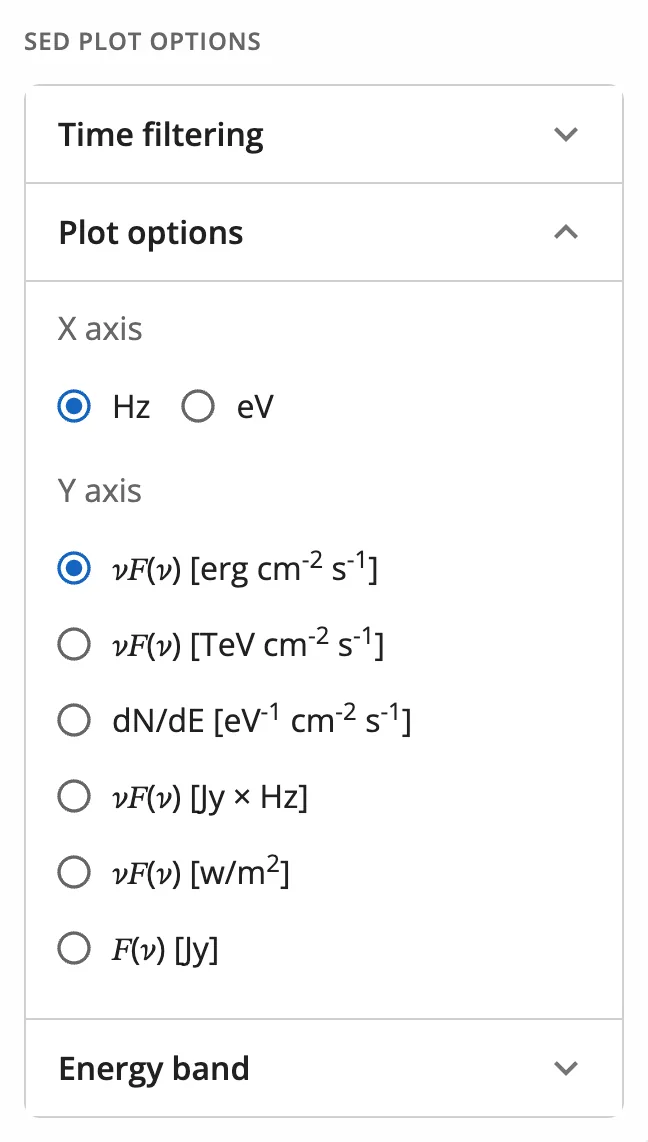
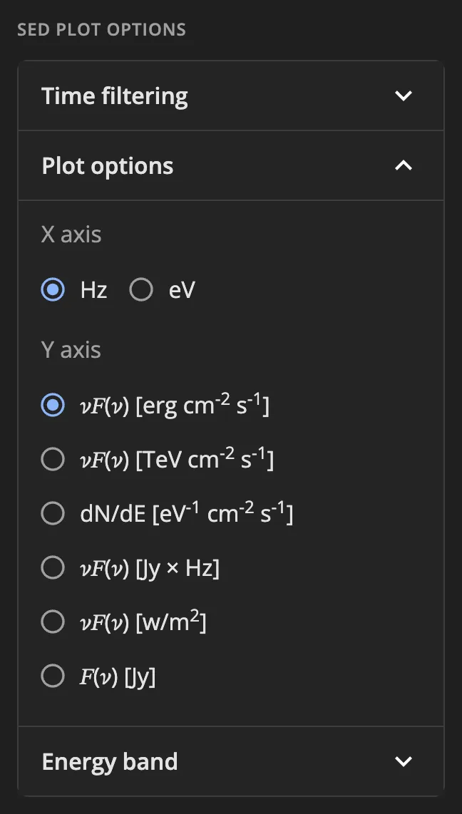
Plot options change the units:

X axis: frequency in Hz, or energy in eV.
Y axis: νF(ν) in erg cm⁻² s⁻¹, TeV cm⁻² s⁻¹, Jy × Hz or W/m², dN/dE in eV⁻¹ cm⁻² s⁻¹, or F(ν) in Jy.

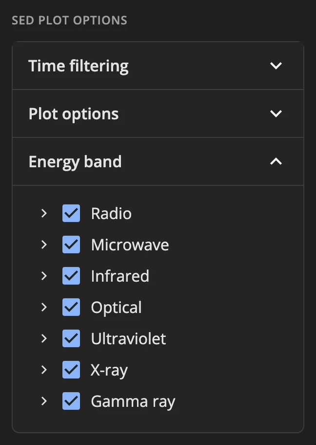
Energy band lists the bands (radio to gamma rays) and, inside each, the catalogues that returned data. Untick a band or a catalogue to hide its points.

The options apply to the SED tab.

4. Download the data¶

The CSV (Hz, erg cm⁻² s⁻¹) button in the source card downloads the points shown: it follows the time window and the ticked catalogues. Units are always Hz and erg cm⁻² s⁻¹, whatever the axes on screen.

Column	Content
`freq_hz`	Frequency [Hz]
`nufnu`	νF(ν) [erg cm⁻² s⁻¹]
`nufnu_err`	Error on νF(ν) [erg cm⁻² s⁻¹]
`is_ul`	`true` if the point is an upper limit
`mjd_start`	Start of the observation [MJD]; empty when unknown
`mjd_end`	End of the observation [MJD]; empty when unknown
`catalog`	Catalogue the point comes from
`band`	Energy band
`reference`	Bibliographic reference of the catalogue

Every row carries its reference, so the data can be cited properly. MMDC data are available under CC BY 4.0; see Citing.

5. More about the source¶

The tabs above the plot open once a source is plotted.

SED/LC animation¶

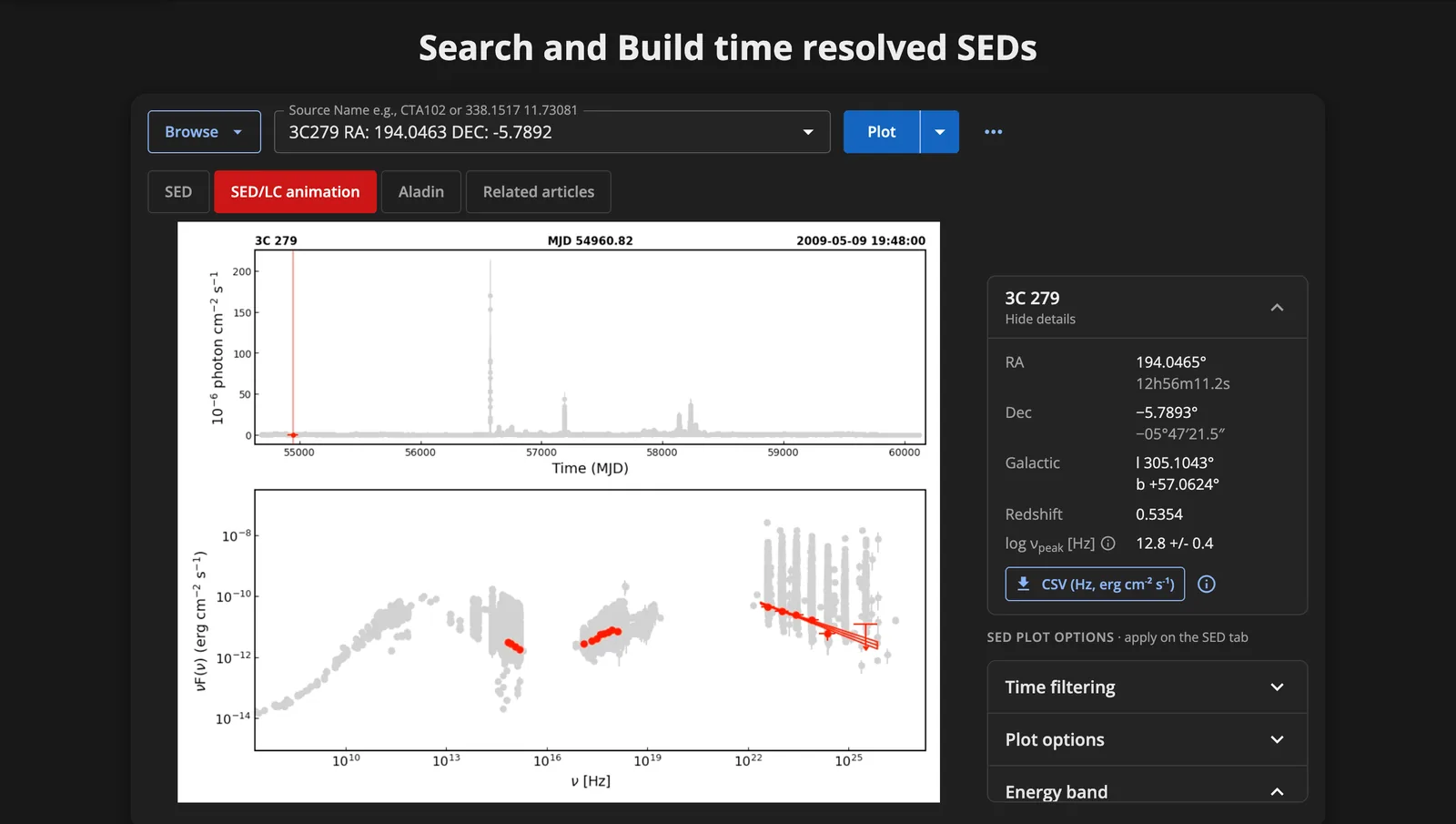
A video of how the SED changes over time, built from quasi-simultaneous data, next to the light curve. It is pre-computed for a set of sources; for the others the tab says the animation is not available.

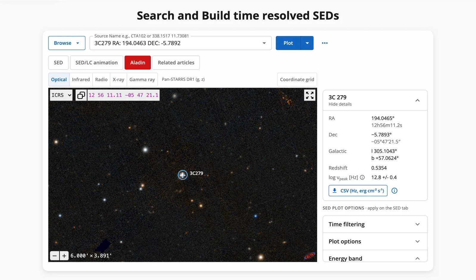
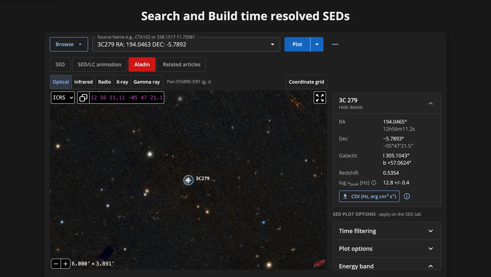
Aladin¶

The sky around the source in the Aladin Lite atlas, with the source marked. Switch between optical, infrared, radio, X-ray and gamma-ray surveys, and turn on a coordinate grid. It needs a browser with WebGL2.

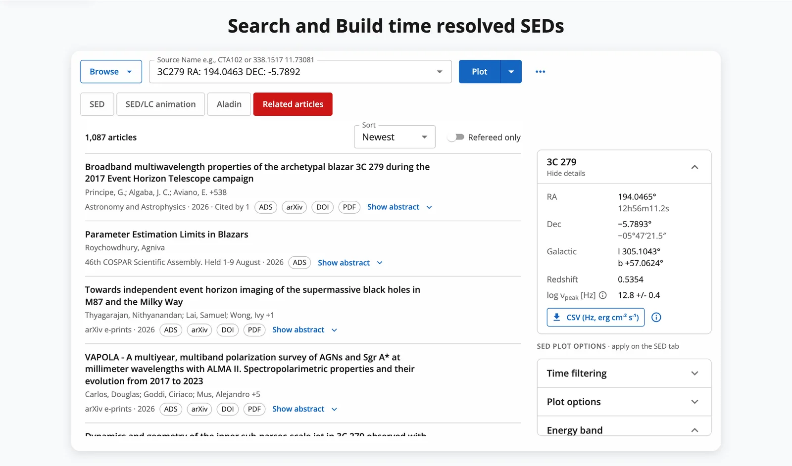
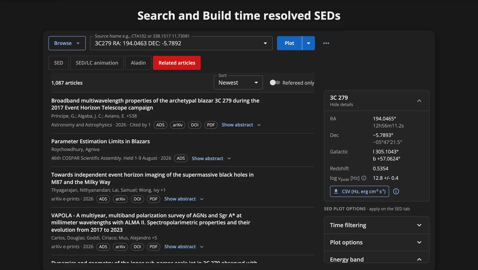
Papers about the source from the SAO/NASA Astrophysics Data System (ADS). Sort by Newest, Most cited or Relevance, keep only refereed papers, open an abstract, and follow the ADS, arXiv, DOI and PDF links.

From Python¶

Everything on this page is also available from Python with the astro-mmdc SDK: see SED data.